using Revise
using LinearAlgebra
using BenchmarkTools
using EcologicalNetworks
using NetworkDiagonality
using Plots
using SparseArrays
using StatsBase
Read the previous episodes here: - Part 1 - Part 2 - Part 3
Starting to package code
I’ve started to package some code, not yet a full package, but first steps. You can find the work-in-progress package on a gitlab repository: please DO contribute if you feel like it!
Where’s your mass now?
I had a chat with Chris Price, Linear Algebra and Optimization guru here at UC. He said he had “bad” news for me. But they were not so bad.
The problem we are facing, according to his gut, seems a nice hard one. It resembles a bit the Traveling Sales Agent problem. But with additional nastiness.
Chris also suggest a complimentary (or alternative) way of speeding up our research of a good (if not best) diagonality representation for a network. The idea is to 1. first compute for each row where its “centre of mass” is: that is, where are the ones concentrated? Toward the end or the start of the row? 2. then, we can sort the rows according to their centre of mass, so that rows that have most ones at the end of the row are at the bottom of the matrix, and the one with more ones in the middle are in the middle. This roughly should put the ones over the diagonal. 3. we do the same, but for columns; 4. and iterate 1. to 3. until we reach some convergence (IF we reach some convergence).
The complexity of Chris’ approach seems much lower, and we can use it either in isolation or to improve the mesh refinement step.
A quick implementation of Chris’ idea
Let’s take one of our test matrices (by the way, we have been working a lot with Jarrod D Hadfield, Boris R. Krasnov, Robert Poulin and Shinichi Nakagawa 2013’s A tale of two phylogenies: comparative analyses of ecological interactions that you can find in The American Naturalist, big shoutout to them!).
Net = get_binet_wol(10);
A = get_sadj_net(Net)
31×18 SparseMatrixCSC{Int64,Int64} with 88 stored entries:
[1 , 1] = 1
[2 , 1] = 1
[3 , 1] = 1
[4 , 1] = 1
[6 , 1] = 1
[8 , 1] = 1
[9 , 1] = 1
[10, 1] = 1
[16, 1] = 1
⋮
[20, 14] = 1
[7 , 15] = 1
[14, 15] = 1
[4 , 16] = 1
[11, 16] = 1
[1 , 17] = 1
[7 , 17] = 1
[11, 17] = 1
[14, 17] = 1
[6 , 18] = 1
we get row and col size (we are going to use those a lot):
R,C = size(A)(31, 18)
and let’s take another look at it:
hm(A::T) where T <: AbstractSparseMatrix = heatmap(Matrix(A), yflip = true)
hm(A)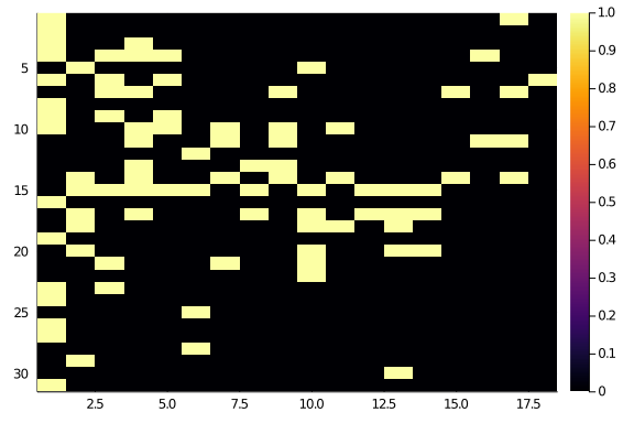
and let’s consider a couple of “easy” rows, say i = 23 and
i = 21:
hm(A[[21,23], :])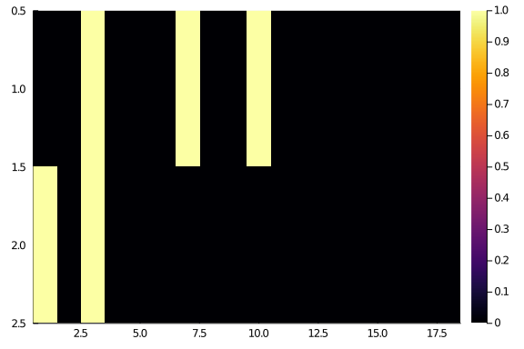
the first row (row 21) has interactions with columns 3, 7, and 10; the second one (row 23) has interactions with columns 1 and 3. So, it makes more sense to put row 21 after row 23, if we want to see a “diagonal” matrix. And we can make the same reasonment for every row and column.
The simplest approach is to compute the average position of the 1s in each row. To do it, we are going to convert the sparse row into a dense vector (it will be useful later on).
function centre_mass(A_vec::T) where T <: SparseVector
    dense_vec = Vector(A_vec)
    where_not_zero = collect(1:length(dense_vec))[dense_vec .> 0]
    return sum(where_not_zero)/length(where_not_zero)
end
centre_mass (generic function with 1 method)
Notice: we will need to think about what to do with completely empty rows and / or columns. We can apply the function to every row:
row_rank = Array{Float64}(undef, R)
for row in 1:R
    row_rank[row] = centre_mass(A[row,:])
end
and then sort the rows accordingly:
new_row_order = sortperm(row_rank)
newA = permute(A,new_row_order,collect(1:C))
31×18 SparseMatrixCSC{Int64,Int64} with 88 stored entries:
[1 , 1] = 1
[2 , 1] = 1
[3 , 1] = 1
[4 , 1] = 1
[5 , 1] = 1
[6 , 1] = 1
[7 , 1] = 1
[8 , 1] = 1
[9 , 1] = 1
⋮
[28, 14] = 1
[26, 15] = 1
[27, 15] = 1
[13, 16] = 1
[30, 16] = 1
[23, 17] = 1
[26, 17] = 1
[27, 17] = 1
[30, 17] = 1
[20, 18] = 1
The operation has given back something more diagonal:
hm(newA)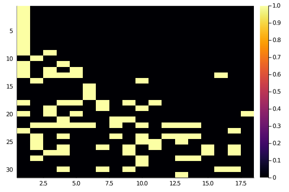
We can then operate on the columns similarly:
col_rank = Array{Float64}(undef,C)
for col in 1:C
    col_rank[col] = centre_mass(newA[:,col])
end

new_col_order = sortperm(col_rank)
newA .= permute(newA,collect(1:R),new_col_order)
31×18 SparseMatrixCSC{Int64,Int64} with 88 stored entries:
[1 , 1] = 1
[2 , 1] = 1
[3 , 1] = 1
[4 , 1] = 1
[5 , 1] = 1
[6 , 1] = 1
[7 , 1] = 1
[8 , 1] = 1
[9 , 1] = 1
⋮
[24, 16] = 1
[25, 16] = 1
[28, 16] = 1
[31, 16] = 1
[26, 17] = 1
[27, 17] = 1
[23, 18] = 1
[26, 18] = 1
[27, 18] = 1
[30, 18] = 1
hm(newA)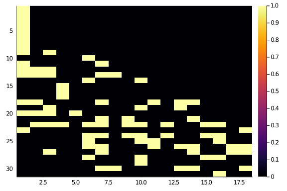
Even better (a part from that start of 1s, which could probably go in the middle, don’t they?).
Repeating a couple (well, a 100 couples) of time, keeping trace of how many rows we actually moved around.
moves = zeros(Int,200,2)
for x in 1:200
    row_rank = Array{Float64}(undef, R)
    for row in 1:R
    @inbounds row_rank[row] = centre_mass(newA[row,:])
    end
    new_row_order = sortperm(row_rank)
    moves[x,1] = sum(new_row_order .!=   1:R)
    newA .= permute(newA,new_row_order,collect(1:C))

    col_rank = Array{Float64}(undef,C)
    for col in 1:C
    @inbounds  col_rank[col] = centre_mass(newA[:,col])
    end
    new_col_order = sortperm(col_rank)
    moves[x,2] = sum(new_col_order .!=   1:C)
    newA .= permute(newA,collect(1:R),new_col_order)

end
And let’s take a look
hm(newA)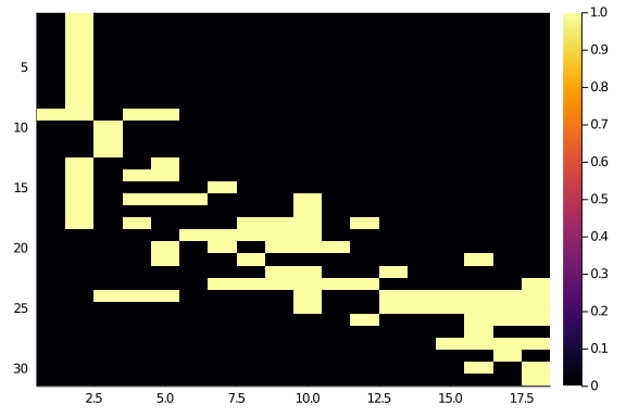
Not too bad at all, although not perfect. And it actually reached a stable configuration quite quickly (less than 10 steps).
plot(1:15,moves[1:15,1])
plot!(1:15,moves[1:15,2])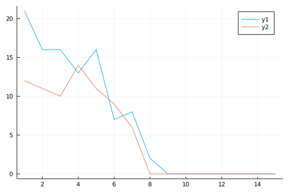
Cool, let’s see how fast that is (we should reshuffle the matrix we start from) using the function we wrapped up in the package.
max_steps = 200

@benchmark cm_optimization_diag!($shuffle(A),$max_steps)
BenchmarkTools.Trial:
memory estimate: 389.16 KiB
allocs estimate: 3958
--------------
minimum time: 244.096 μs (0.00% GC)
median time: 544.789 μs (0.00% GC)
mean time: 727.098 μs (18.79% GC)
maximum time: 18.409 ms (93.59% GC)
--------------
samples: 6872
evals/sample: 1
Much faster than the simulated annealing, yet this also only provides a quite worse result. It seems something we can take advantage of, bringing the network in a better configuration before starting the simulate annealing. And maybe after some work on the reduce resolution grids.
Blurring
Now, on to the blurring idea. To recap the plan: instead of working directly on the observed adjacency matrix, which is huge, we are going to summarise it in a much smaller matrix, where we can explore more of the row/column order space. Then, we’ll move on gradually to higher resolution. This should ensure a much better starting post for the final, full resolution, simulated annealing.
Squinting
The first step requires a function to produce the lower resolution matrices. The
key steps here are the ability of partitioning an array of indexes of balanced
(if not equal) size. Luckily, the Iterator module offers the right function with
Iterators.partition().
For example, let’s consider a matrix with 200 rows, and let’s try to produce 17
chunks. That means that each chunk should have rougly 200⁄17 elements. But 20 is not
divisible by 17. No problem! We can use cld(x,y) to get the “smallest integer larger
than or equal to x/y”. Then, Iterators.partition() will split the arrays of indexes
of at most that many elements.
With an example:
Row_number = 200
How_many_pieces = 17

Row_indexes = 1:1:Row_number
Row_chunks = Iterators.partition(Row_indexes, cld(Row_number,How_many_pieces)) |>
    collect
17-element Array{StepRange{Int64,Int64},1}:
1:1:12
13:1:24
25:1:36
37:1:48
49:1:60
61:1:72
73:1:84
85:1:96
97:1:108
109:1:120
121:1:132
133:1:144
145:1:156
157:1:168
169:1:180
181:1:192
193:1:200
The length of the chunks are balanced:
countmap(length.(Row_chunks))Dict{Int64,Int64} with 2 entries:
8 => 1
12 => 16
And we get for free the ability to chunk up array of indexes that have been shuffled up:
Row_indexes = sample(1:1:Row_number, Row_number, replace = false)
Row_chunks = Iterators.partition(Row_indexes, cld(Row_number,How_many_pieces)) |>
    collect
17-element Array{SubArray{Int64,1,Array{Int64,1},Tuple{UnitRange{Int64}},tr
ue},1}:
[32, 4, 1, 161, 163, 84, 55, 164, 81, 59, 110, 19]
[23, 49, 117, 29, 119, 8, 180, 149, 200, 128, 80, 111]
[130, 97, 166, 181, 178, 5, 144, 150, 195, 103, 85, 83]
[136, 92, 162, 120, 17, 132, 56, 68, 191, 46, 65, 86]
[43, 64, 190, 60, 6, 186, 127, 146, 123, 12, 122, 151]
[171, 99, 89, 176, 125, 22, 107, 25, 189, 63, 145, 13]
[67, 14, 133, 184, 148, 193, 91, 112, 131, 24, 197, 169]
[34, 7, 54, 173, 175, 48, 121, 183, 199, 87, 45, 77]
[165, 57, 142, 152, 40, 139, 58, 138, 31, 179, 137, 10]
[39, 116, 172, 94, 44, 41, 141, 90, 100, 106, 30, 158]
[182, 69, 159, 129, 124, 170, 160, 118, 192, 27, 62, 174]
[79, 155, 187, 93, 168, 42, 51, 167, 3, 115, 108, 72]
[101, 47, 102, 26, 71, 196, 88, 52, 157, 61, 2, 153]
[185, 70, 15, 28, 194, 114, 21, 96, 82, 104, 16, 147]
[73, 37, 66, 9, 76, 74, 95, 38, 113, 75, 156, 198]
[135, 78, 50, 177, 105, 18, 33, 188, 154, 140, 134, 143]
[36, 35, 53, 11, 98, 20, 126, 109]
Once we are able to partition the indexes, we sum up all the entries in a row/column chunk of the original matrix. We do this looping over all the chunks.
In the package we have coded everything into a function. So, let’s create 2×2,
3×3, and 4×5 resolution versions of A. To emphasize what’s happening, we
start from a shuffled A.
A = shuffle(A)
# lower_resolution also returns the indexes partitions
A₂₂, _, _ = lower_resolution(A,2,2)
A₃₃, _, _ = lower_resolution(A,3,3)
A₄₅, _, _ = lower_resolution(A,4,5)
plot(layout = (2,2),
    hm(A),
    hm(A₂₂),
    hm(A₃₃),
    hm(A₄₅))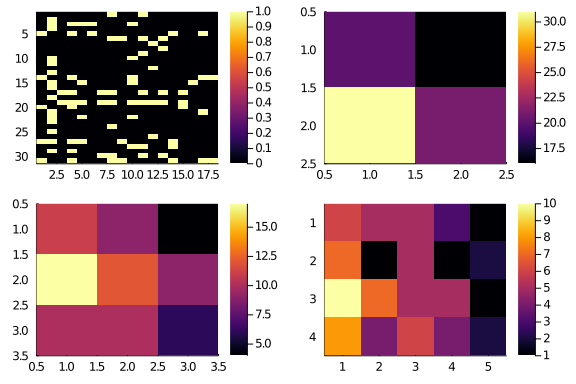
Sorting the lows
The next step is to optimize the representation of the lower resolution matrices. Luckily, the diagonal score function we coded up works fine also on this non binary function. A part from the normalization, which we can skip if we only care about maximising the diagonality (by setting an appropriate target for the simulated annealing).
We start with our 4×5 low resolution matrix, and get a matrix of diagonal scores of the right size, so we can compute the starting point diagonality:
A₄₅, Rchunks, Cchunks = lower_resolution(A,4,5)
Scores₄₅ = diagonal_scores(size(A₄₅)...)
obs_diag_lowr = diagonality(A₄₅,Scores₄₅)
19.0
Then, we reorder the rows of A₄₅ so to increase its diagonality. We choose a target of twice the observed diagonality: we don’t need to get it perfectely right. And, because of the small size of the matrix we are operating on, we can take just a couple of hundred steps.
new_rows, new_columns = sa_optimization_diag(A₄₅,
        Scores₄₅,
        target = 2 * obs_diag_lowr,
        Nsteps = 200)
([2, 3, 1, 4], [5, 2, 1, 3, 4])
We are going to use the new row and column order to permute our low resolution matrix. Let’s see how that would look like
score_plot = hm(Scores₄₅);
title!(score_plot,"Scores");

lowr_plot = hm(A₄₅);
title!(lowr_plot,"Low Resolution");

permuted_plot =  heatmap(
        string.(new_columns),
        string.(new_rows),
        Matrix(permute(A₄₅,new_rows,new_columns)),
        yflip = true,
        title = "Permuted");

plot(
score_plot,
lowr_plot,
permuted_plot
)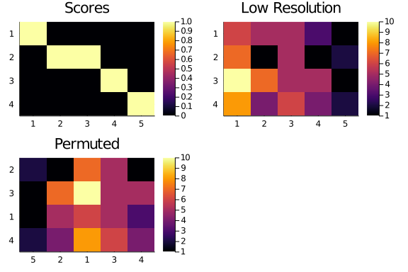
The improvement may not be immediately visible, but we can compare the previous diagonality value with the one for the permuted low resolution matrix.
diagonality(permute(A₄₅,new_rows,new_columns),Scores₄₅)28.0
A good improvement!
Squinting, then reordering
The final step is to propagate the optimization up to the highest resolution.
The delicate part is to keep track of the indexes properly: once we reordered some at the lower resolution level, we need to update the ones at the original resolution. We can do this by concatening the chunks in the right order:
new_R_indexes = vcat([Rchunks[i] for i in new_rows]...)
new_C_indexes = vcat([Cchunks[i] for i in new_columns]...)
18-element Array{Int64,1}:
17
18
5
6
7
8
1
2
3
4
9
10
11
12
13
14
15
16
We can now use the new indexes to permute our observed matrix. We compare the original and the permuted matrices for reference:
A_hm = heatmap(
        string.(1:size(A)[2]),
        string.(1:size(A)[1]),
        Matrix(A),
        yflip = true)
newA_hm = heatmap(
        string.(new_C_indexes),
        string.(new_R_indexes),
        Matrix(permute(A,new_R_indexes,new_C_indexes)),
        yflip = true)
plot(
    A_hm,
    newA_hm
)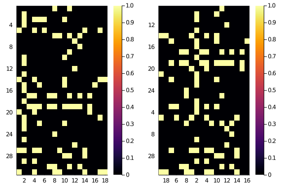
For a double check, we can test whether the low resolution reordering has actually improved the high resolution diagonality:
We started from
diagonality(A,
    diagonal_scores(size(A)...))
21.103003409430492
and now we are at
diagonality(
    permute(A,new_R_indexes,new_C_indexes),
    diagonal_scores(size(A)...))
28.117676440736666
Which doesn’t sound like a lot, but it’s in the right direction.
In the next blogpost we are going to pull all our weaponry together and tackle some real ecological analysis. Finally. I hope. 😸